Modern computers tend to have multiple processors. By making use of all the processing ability of your machine your programs can run much faster. Writing code that takes advantage of multiple processors in Java usually involves either manually creating and managing threads, or using a higher level concurrent programming abstraction library, such as the classes found in the excellent java.util.concurrent package.

A common use-case for multithreading in multimedia analysis is the application of an operation to a collection of objects - for example, the extraction of features from a list of images. This kind of task can be effectively parallelised using Java’s concurrent classes, but requires a large amount of boiler-plate code to be written each time. To help reduce the programming overhead associated with this kind of parallel processing, OpenIMAJ includes a Parallel class that contains a number of methods that allow you to efficiently and effectively write multi-threaded loops.

To get started playing with the Parallel class, create a new OpenIMAJ project using the archetype, or add a new class and main method to an existing project. Firstly, lets see how we can write the parallel equivalent of a for (int i=0; i<10; i++) loop:

Parallel.forIndex(0, 10, 1, new Operation<Integer>() {
	public void perform(Integer i) {
	    System.out.println(i);
	}
});

Try running this code; you’ll see that all the numbers from 0 to 9 are printed, although not necessarily in the correct order. If you run the code again, you’ll probably see the order change. It’s important to note that the when parallelising a loop that the order of operations is not deterministic.

Now let’s explore a more realistic scenario in which we might want to apply parallelisation. We’ll build a program to compute the normalised average of the images in a dataset. Firstly, let’s write the non-parallel version of the code. We’ll start by loading a dataset of images; in this case we’ll use the CalTech 101 dataset we used in the Classification 101 tutorial, but rather than loading record object, we’ll load the images directly:

VFSGroupDataset<MBFImage> allImages = Caltech101.getImages(ImageUtilities.MBFIMAGE_READER);

We’ll also restrict ourselves to using a subset of the first 8 groups (image categories) in the dataset:

GroupedDataset<String, ListDataset<MBFImage>, MBFImage> images = GroupSampler.sample(allImages, 8, false);

We now want to do the processing. For each group we want to build the average image. We do this by looping through the images in the group, resampling and normalising each image before drawing it in the centre of a white image, and then adding the result to an accumulator. At the end of the loop we divide the accumulated image by the number of samples used to create it. The code to perform these operations would look like this:

List<MBFImage> output = new ArrayList<MBFImage>();
ResizeProcessor resize = new ResizeProcessor(200);
for (ListDataset<MBFImage> clzImages : images.values()) {
    MBFImage current = new MBFImage(200, 200, ColourSpace.RGB);

    for (MBFImage i : clzImages) {
        MBFImage tmp = new MBFImage(200, 200, ColourSpace.RGB);
        tmp.fill(RGBColour.WHITE);

        MBFImage small = i.process(resize).normalise();
        int x = (200 - small.getWidth()) / 2;
        int y = (200 - small.getHeight()) / 2;
        tmp.drawImage(small, x, y);

        current.addInplace(tmp);
    }
    current.divideInplace((float) clzImages.size());
    output.add(current);
}

We can use the DisplayUtilities class to display the results:

DisplayUtilities.display("Images", output);

Before we try running the program, we’ll also add some timing code to see how long it takes. Before the outer loop (the one over the groups provided by images.values()), add the following:

Timer t1 = Timer.timer();

and, after the outer loop (just before the display code) add the following:

System.out.println("Time: " + t1.duration() + "ms");

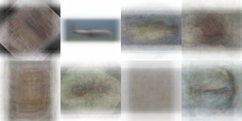
You can now run the code, and after a short while (on my laptop it takes about 7248 milliseconds (7.2 seconds)) the resultant averaged images will be displayed. An example is shown below. Can you tell what object is depicted by each average image? For many object types in the CalTech 101 dataset it is quite easy, and this is one of the reasons that the dataset has been criticised as being too easy for classification experiments in the literature.

Now we’ll look at parallelising this code. We essentially have three options for parallelisation; we could parallelise the outer loop, parallelise the inner one, or parallelise both. There are many tradeoffs that need to be considered including the amount of memory usage and the task granularity in deciding how to best parallelise code. For the purposes of this tutorial, we’ll work with the inner loop. Using the Parallel.for method, we can re-write the inner-loop as follows:

Parallel.forEach(clzImages, new Operation<MBFImage>() {
    public void perform(MBFImage i) {
        final MBFImage tmp = new MBFImage(200, 200, ColourSpace.RGB);
        tmp.fill(RGBColour.WHITE);

        final MBFImage small = i.process(resize).normalise();
        final int x = (200 - small.getWidth()) / 2;
        final int y = (200 - small.getHeight()) / 2;
        tmp.drawImage(small, x, y);

        synchronized (current) {
            current.addInplace(tmp);
        }
    }
});

For this to compile, you’ll also need to make the current image final by adding the final keyword to the line in which it is created:

final MBFImage current = new MBFImage(200, 200, ColourSpace.RGB);

Notice that in the parallel version of the loop we have to put a synchronized block around the part where we accumulate into the current image. This is to stop multiple threads trying to alter the image concurrently. If we now run the code, we should hopefully see an improvement in the time it takes to compute the averages. You might also need to increase the amount of memory available to Java for the program to run successfully.

On my laptop, with 8 CPU cores the running time drops to ~3100 milliseconds. You might be thinking that because we have gone from 1 to 8 CPU cores that the speed-up would be greater; there are many reasons why that is not the case in practice, but the biggest is that the process that we’re running is rather I/O bound because the underlying dataset classes we’re using retrieve the images from disk each time they’re needed. A second issue is that there are a couple of slight bottlenecks in our code; in particular notice that we’re creating a temporary image for each image that we process, and that we also have to synchronise on the current accumulator image for each image. We can factor out these problems by modifying the code to use the partitioned variant of the for-each loop in the Parallel class. Instead of giving each thread a single image at a time, the partitioned variant will feed each thread a collection of images (provided as an Iterator) to process:

Parallel.forEachPartitioned(new RangePartitioner<MBFImage>(clzImages), new Operation<Iterator<MBFImage>>() {
	public void perform(Iterator<MBFImage> it) {
	    MBFImage tmpAccum = new MBFImage(200, 200, 3);
	    MBFImage tmp = new MBFImage(200, 200, ColourSpace.RGB);

	    while (it.hasNext()) {
	        final MBFImage i = it.next();
	        tmp.fill(RGBColour.WHITE);

	        final MBFImage small = i.process(resize).normalise();
	        final int x = (200 - small.getWidth()) / 2;
	        final int y = (200 - small.getHeight()) / 2;
	        tmp.drawImage(small, x, y);
	        tmpAccum.addInplace(tmp);
	    }
	    synchronized (current) {
	        current.addInplace(tmpAccum);
	    }
	}
});

The RangePartitioner in the above code will break the images in clzImages into as many (approximately equally sized) chunks as there are available CPU cores. This means that the perform method will be called many fewer times, but will do more work - what we’ve done is called increasing the task granularity. Notice that we created an extra working image called tmpAccum to hold the intermediary results. This means memory usage will be increased, however, also notice that whilst we still have to synchronise on the current image, we do far fewer times (once per CPU core in fact). Try running the improved version of the code; on my laptop it reduces the total running time even further to ~2900 milliseconds.