Let's dive straight in and get something going before we look at some audio theory and more complex audio processing. One of the most useful things to do with audio is to listen to it! Playing an audio file in OpenIMAJ is very easy: simply create your audio source and pass it to the audio player.

XuggleAudio xa = new XuggleAudio( new File( "myAudioFile.mp3" ) );
AudioPlayer.createAudioPlayer( xa ).run();

If you run these 2 lines of code you should hear audio playing. The XuggleAudio class uses the Xuggler library to decode the audio from the file. The audio player ()that's constructed using a static method as with the video player) returns an audio player instance which we set running straight away.

What's happening underneath is that the Xuggler library decodes the audio stream into chunks of audio (called frames) each of which has many samples. A sample represents a level of sound pressure and the more of these there are within one second, the better the representation of the original continuous signal. The number of samples in one second is called the sample rate and you may already know that audio on CDs are encoded at 44,100 samples per second (or 44.1KHz). The maximum frequency that can be encoded in a digital signal is half of the sample rate (e.g. an estimate of a 22.05KHz sine wave with a 44.1KHz sampled signal will be {1,-1,1,-1...}). This is called the Nyquist frequency (named after Swedish-American engineer Harry Nyquist).

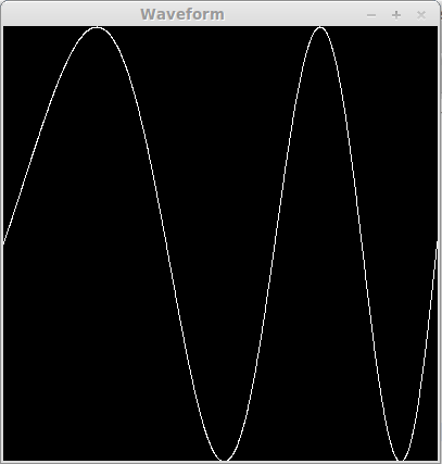
Let's have a look at the audio waveform. This is easy to do with OpenIMAJ as we have a subproject that contains various visualisers for various data including audio data. The AudioWaveform visualisation acts as a very basic oscilloscope for displaying the audio data. We'll use a file from http://audiocheck.net/ as it's good for understanding some of the audio functions we're about to describe. We can link directly to the file by passing a URL to XuggleAudio (as in the code snippet below) or you can download the 20Hz-20KHz sweep and use it by passing a File to the XuggleAudio.

final AudioWaveform vis = new AudioWaveform( 400, 400 );
vis.showWindow( "Waveform" );

final XuggleAudio xa = new XuggleAudio( 
    new URL( "http://www.audiocheck.net/download.php?" +
        "filename=Audio/audiocheck.net_sweep20-20klin.wav" ) );

SampleChunk sc = null;
while( (sc = xa.nextSampleChunk()) != null )
    vis.setData( sc.getSampleBuffer() );

So, the first two lines above create the visualisation. We open the file and then we iterate through the audio stream (with xa.nextSampleChunk()) and send that data to the visualisation (we'll cover the getSampleBuffer() method later).

The audio subsystem in OpenIMAJ has been designed to match the programming paradigm of the image and video subprojects. So, all classes providing audio extend the Audio class. Currently all implementations also extend the AudioStream class which defines a method for getting frames of audio from the stream which we call SampleChunks in OpenIMAJ. A SampleChunk is a wrapper around an array of bytes. Understanding what those bytes mean requires knowledge of the format of the audio data and this is given by the AudioFormat class.

Audio data, like image data, can come in many formats. Each digitised reading of the sound pressure (the sample) can be represented by 8 bits (1 byte, signed or unsigned), 16 bits (2 bytes, little or big endian, signed or unsigned), or 24 bits or more. The sample rate can be anything, although 22.05KHz or 44.1KHz is common for audio (48KHz for video). The audio data can also represent one (mono), two (stereo) or more channels of audio, which are interleaved in the sample chunk data.

To make code agnostic to the audio format, OpenIMAJ has a API that provides a means for accessing the sample data in a consistent way. This class is called a SampleBuffer. It has a get(index) method which returns a sample as a value between 0..1 whatever the underlying size of the data. It also provides a set(index,val) method which provides the opposite conversion. Multichannel audio is still interleaved in the SampleBuffer, however, it does provide various accessors for getting data from specific channels. An appropriate SampleBuffer for the audio data in a SampleChunk can be retrieved using SampleChunk.getSampleBuffer().

Ok, enough theory for the moment. Let's do something interesting that will help us towards understanding what we're getting in.

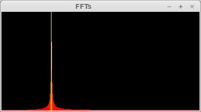
An algorithm called the Fourier Transform converts a time-domain signal (i.e. the signal you're getting from the audio file) into a frequency-domain signal (describing what pitches or frequencies contribute towards the final signal). We can see what frequencies are in our signal by applying the transform and visualising the results.

Take the previous code and change the visualisation to be a BarVisualisation. Next, we'll create a FourierTransform object and take our stream of data from there.

FourierTransform fft = new FourierTransform( xa );
...
while( (sc = fft.nextSampleChunk()) != null )
{
    float[][] fftData = fft.getMagnitudes();
    vis.setData( fftData[0] );
}

Run this demo on the audiocheck.net sine wave sweep and you'll see a peak in the graph moving up through the frequencies. The lowest frequencies are on the left of the visualisation and the highest frequencies on the right (the Nyquist frequency on the far right).

This example also introduces us to the processor chaining in the OpenIMAJ audio system. Chaining allows us to create a set of operations to apply to the audio data and to take the final data stream from the end. In this case we have chained the FourierTransform processor to the original audio stream and we're taking the data from the end of the stream, as shown in the diagram below.

When we call nextSampleChunk() on the FourierTransform object, it goes and gets the sample chunk from the previous processor in the chain, processes the sample chunk and returns a new sample chunk (in fact, the FourierTransform returns the sample chunk unchanged).

Let's put an EQ filter in the chain that will filter out frequencies from the original signal:

EQFilter eq = new EQFilter( xa, EQType.LPF, 5000 );
FourierTransform fft = new FourierTransform( eq );

We have set the low-pass filter (only lets low frequencies through) to 5KHz (5000Hz), so when you run the program again, you will see the peak fall off some way along its trip up to the high frequencies. This sort of filtering can be useful in some circumstances for directing processing to specific parts of the audio spectrum.

So, we've learned a bit about audio, seen the basics of the audio subsystem in OpenIMAJ and even started looking into the audio. In the next chapter, we'll start extracting features and trying to do something interesting with it, bringing in other parts of the OpenIMAJ system.